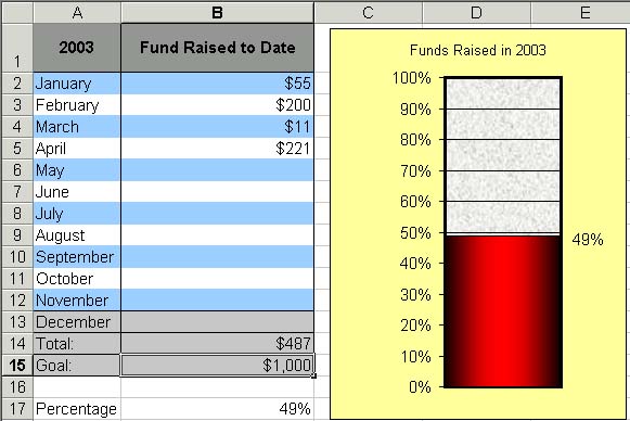
Make a thermometer style chart like the one displayed at the bottom of the page!


This chart will track the daily progress toward a goal. In this case, a goal of $1,000.

Cell B15 contains the Goal Value. Cell B14 contains the sum formula: =SUM(B2:B12)

As data is entered into column B, the chart is automatically updated to reflect the changes.

To create the chart:
1. Enter the formulas listed above, along with the worksheet's sample data.
2. Select cell B17, and click the Chart Wizard button.
3. In step 1 of the Chart Wizard dialog, specify a Column chart and a Clustered Column subtype (the first choice).
4. Click Next twice, and then in step 2 make additional adjustments: Add a chart title (Title Tab), dump the Category (X) axis (Axes tab), delete the legend (Legend tab), and specify Show value (Data Labels tab). Click Finish to view the chart.
5. Double-click the column to display the Format Data Series dialog box.
6. Click the Options tab, and set the Gap width to ) (this setting instructs the column to occupy the entire width of the plot area).
7. To change the pattern used in the column, click the Patterns tab and make your selection. The example shown here uses a gradient fill effect.
8. Double-click the vertical axis to bring up the Format Axis dialog. In the Scale tab of the Format Axis dialog, set Minimum to ) and Maximum to 1.

If you would like to change any of the chart parameters at any time, right click on the chart and select the appropriate option.