Welcome to Wally's Spreadsheet Page I seem to use Excel on a daily basis. I recently decided to create a space where I could share some of the spreadsheet information that I have garnered over the past year or two. I hope this is helpful.

Functions Functions are the workhorse of Excel. They allow a user to perform numerous calculations on data. Functions run the gamut from simple functions that will sum a column of numbers to complex functions that lookup and perform calculations on data from websites.

The Concatenate Function

This function will allow you to put together two or more text strings. As an example, you design a worksheet to include cell A1 as a place for a user to type their name. Cell B1 could then contain the formula ="Welcome, "&A1&" to my Excel page."



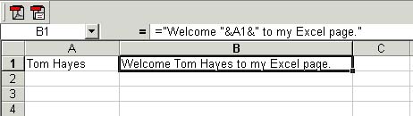
After you enter the formula, click Enter. Cell B2 should read Welcome, (Name) to my Excel page. This formula is especially helpful in querying data from various locations in worksheets and on the web to display in a single placeholder

Macro to change a text string to title case.

This macro is one that I find very handy at times. It will convert a text string to title case, capitalizing the first letter of each word in the string.

Sub TitleCase()
Dim cell As Range
For Each cell In Selection.Cells
If cell.HasFormula = False Then
cell = Application.Proper(cell)
End If
Next
End Sub

Conditional Formatting

Conditional Formatting is another aspect of Excel that can alert you to certain predetermined conditions that occur in a spreadsheet. It is located in the Main Menu under Format.

When you select Conditional Formatting a pop-up window will appear which lets you select conditions to check for in a spreadsheet. As an example, select a range of cells, select Conditional Formatting, select Cell Value, Greater Than, and type a number in the next field. Click Format. Select the Patterns tab, select a Color and click OK. Click OK again. What you should see is for any cell with a number greater than the number you typed in the condition.

Another way to use Conditional Formatting is to use formulas. This formula will create alternating rows of colored rows.

Go to Conditional Formatting and select Formula Is: from the Condition 1 drop-down. Type in the following formula:

=MOD(ROW(Array),2)=0

The array in the formula is the cell range, say a1:b20.

Click Format, the Patterns tab, and select a color. Click OK. Click OK again. What should appear in your spreadsheet is alternating rows of the color you selected for the cells in your array.

If you want two different colors to appear for the cell range, select your cell range, go back to Conditional Formatting, click the Add>> button, and type the following formula as your second condition:

=MOD(ROW(Array),2)=1

Pick a second color from the Pattern tab and click OK twice.

What I really like about this method of coloring rows is it is easy to pick out data, and if I sort the rows, the row colors remain the same.